Hello, World! Let's Recognize Numbers
Index
- Neural Networks
- Backpropagation
- Machine Learning
- MNIST Number Classification (You are here)
The last part was a lot of dry model types and data... Let's put that theory to use and build a Hello, World application of ML, Using MNIST to recognize numbers.
Now, MNIST stands for Modified National Institute of Standards and Technology. These people have spent time and effort labelling 50000+ images of handwritten digits so people like us can use it for machine learning and various other purposes. Now I know I promised we would write code for this blog so here we go, Let's write a digit classifier for these handwritten database of 28px x 28px number images.
Prerequisites
This blog assumes you have basic knowledge of working with Python and Virtual Environments.
Create a working directory for your project and initialize a virutalenv like shown:
python3 -m venv .venvActivate this environment and once you're in it, let's install the required packages
pip install pandas numpy scikit-learn tensorflowLet's open a model.py file. This will serve to create our model and train it with our mnist data. The only imports we need are as follows:
import numpy as np
from sklearn.datasets import fetch_openml
from sklearn.model_selection import train_test_split
from tensorflow import keras
Now conveniently, scikit-learn lets us get the dataset without any additional headaches so all we have to do to fetch our data and split it into training and testing sets is as follows:
def fetch_data():
    X, y = fetch_openml("mnist_784", version=1, return_X_y=True, as_frame=False)

    X_train, X_test, y_train, y_test = train_test_split(
        X, y, test_size=0.2, random_state=42
    )

    y_train = y_train.astype(np.int32)
    y_test = y_test.astype(np.int32)

    return X_train, X_test, y_train, y_test


X_train, X_test, y_train, y_test = fetch_data()
We'll put this as a function since we're going to be reusing this soon enough.
Now we need to design how the model looks, For the sake of simplicity let's use only 3 layers.
- One for flattening the 28x28 image into a vector of length 784
- One hidden layer for processing
- One output layer with 10 neurons to classify digits from 0-9
In code, it will look something like:
model = keras.Sequential(
    [
        keras.layers.Dense(128, activation="relu", input_shape=(784,)),
        keras.layers.Dropout(0.2),
        keras.layers.Dense(64, activation="relu"),
        keras.layers.Dense(10, activation="softmax"),
    ]
)
Notice how we use relu here. If you recall, we talked about this in Part 1.
Now we need to compile our model, just like code, let's do that with some parameters and get a summary of it.
model.compile(
    optimizer="adamax", loss="sparse_categorical_crossentropy", metrics=["accuracy"]
)

model.summary()
The output is going to look something like:
| Layer (type) | Output Shape | Param # |
|---|---|---|
| dense (Dense) | (None, 128) | 100,480 |
| dropout (Dropout) | (None, 128) | 0 |
| dense_1 (Dense) | (None, 64) | 8,256 |
| dense_2 (Dense) | (None, 10) | 650 |
Now let's take our data and train the model with it then save it to a file
history = model.fit(
    X_train, y_train, epochs=10, batch_size=32, validation_split=0.2, verbose=1
)

model.save("mnist.keras")
Feel free to vary the epochs parameter, it refers to how many times is the dataset traversed to learn. For keeping the training time short, let's make it traverse 10 times.
Ok we have a trained model. Now what? We need to measure it's performance and make sure it's actually telling us something useful than spewing gibberish. For that we have to dive into a little bit of math again before we proceed back into code.
Measuring Performance
Precision
Think of precision as "When our model says YES, how often is it actually right?" It's like your friend who loves spotting dogs - if they point at 10 animals saying "That's a dog!" and 7 of those were actually dogs while 3 were cats, their precision would be 7/10 or 70%. In math terms:
Confusion Matrix
Before we jump into F1 score, let's talk about the confusion matrix - it's like a report card for our model showing all the ways it can be right or wrong. Imagine a 2x2 grid:
| Actually Yes | Actually No | |
|---|---|---|
| Model Predicted Yes | TP | FP |
| Model Predicted No | FN | TN |
- True Positives (TP): Model said yes, reality was yes (nailed it!)
- False Positives (FP): Model said yes, reality was no (oops, false alarm)
- False Negatives (FN): Model said no, reality was yes (missed it)
- True Negatives (TN): Model said no, reality was no (correctly ignored)
F1 Score
Now, F1 score is like finding the sweet spot between precision and recall. Recall (also called sensitivity) answers "Out of all actual positive cases, how many did we catch?"
F1 score combines both into a single number:
Think of F1 score as a balanced measure - it's high only when both precision and recall are good. It's especially useful when you have imbalanced classes (like trying to detect rare events) because it takes both false positives and false negatives into account.
A perfect F1 score is 1, meaning your model is spot-on with both precision and recall. A horrible model would score close to 0. Most real-world models fall somewhere in between, and what's considered "good" depends on your specific problem.
Writing code for this
Let's use the help of a couple extra packages to make this beautiful
pip install matplotlib Let's open a test_model.py file where we handle all the forthcoming code. As usual we need imports.
import matplotlib.pyplot as plt
import numpy as np
from sklearn.metrics import confusion_matrix, f1_score, precision_score
from tensorflow import keras
from model import fetch_data
Now let's fetch, prepare and predict our data using the model to evaluate the metrics. Observe how we're just reusing our fetch_data function instead of rewriting it again here.
X_train, X_test, y_train, y_test = fetch_data()

model = keras.models.load_model("mnist.keras")
test_loss, test_accuracy = model.evaluate(X_test, y_test, verbose=0)
print(f"Test accuracy: {test_accuracy:.4f}")

y_pred = model.predict(X_test)
y_pred_classes = np.argmax(y_pred, axis=1)

if len(y_test.shape) > 1:
    y_test_classes = np.argmax(y_test, axis=1)
else:
    y_test_classes = y_test
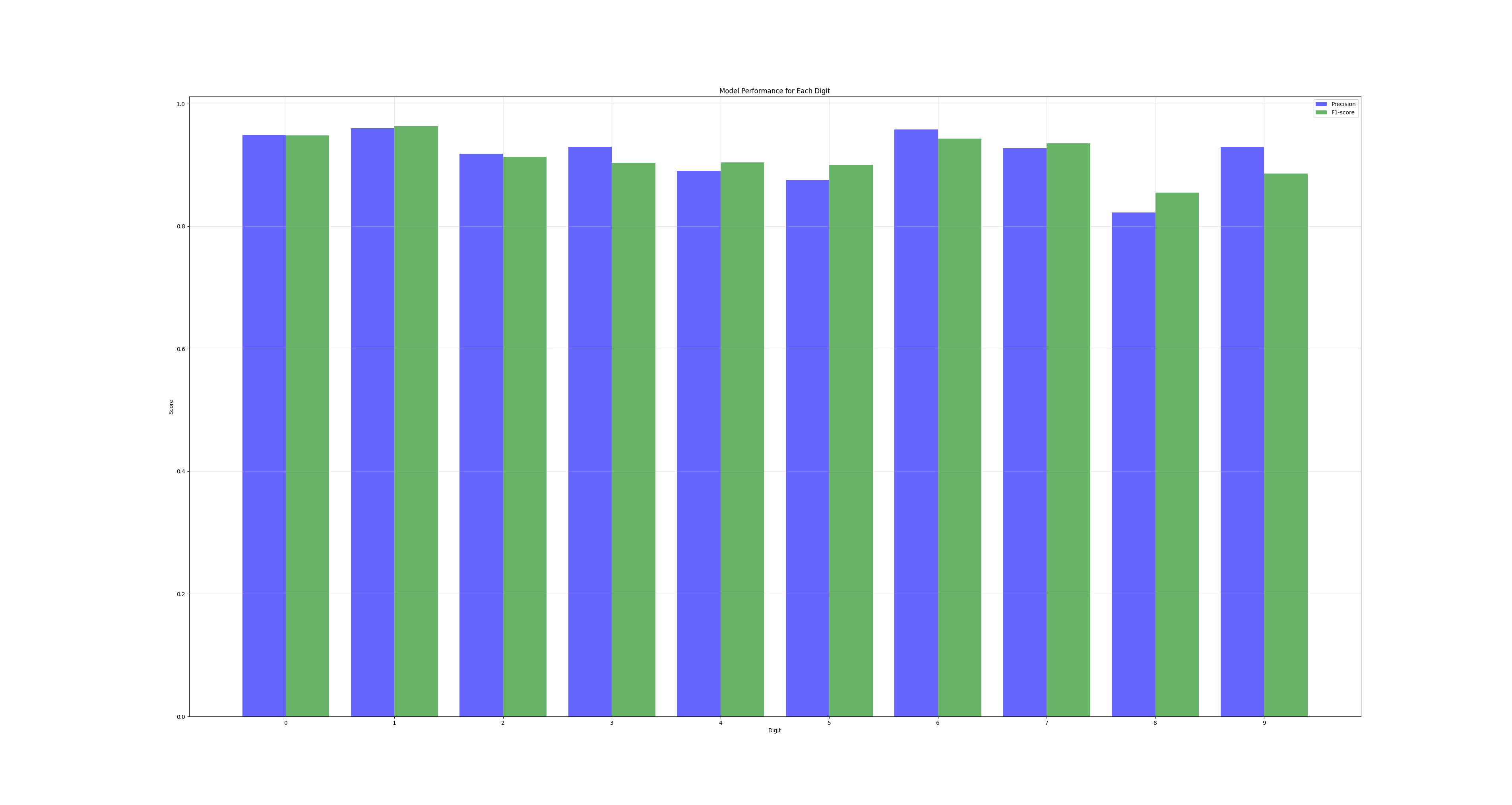
Now using the above snippet, let's plot our precision and F1 score for our model using matplotlib.
precision_per_digit = precision_score(y_test_classes, y_pred_classes, average=None)
f1_per_digit = f1_score(y_test_classes, y_pred_classes, average=None)

plt.figure(figsize=(10, 5))
digits = range(10)  # 0 to 9

plt.bar(
    [x - 0.2 for x in digits],
    precision_per_digit,
    width=0.4,
    label="Precision",
    color="blue",
    alpha=0.6,
)
plt.bar(
    [x + 0.2 for x in digits],
    f1_per_digit,
    width=0.4,
    label="F1-score",
    color="green",
    alpha=0.6,
)

plt.xlabel("Digit")
plt.ylabel("Score")
plt.title("Model Performance for Each Digit")
plt.legend()
plt.grid(True, alpha=0.3)
plt.xticks(digits)

plt.show()
The output is going to look something like this:

Where our blue bars are our precision and green is an f1 score. Right click and open the image in a new tab to see a bigger version of the image.
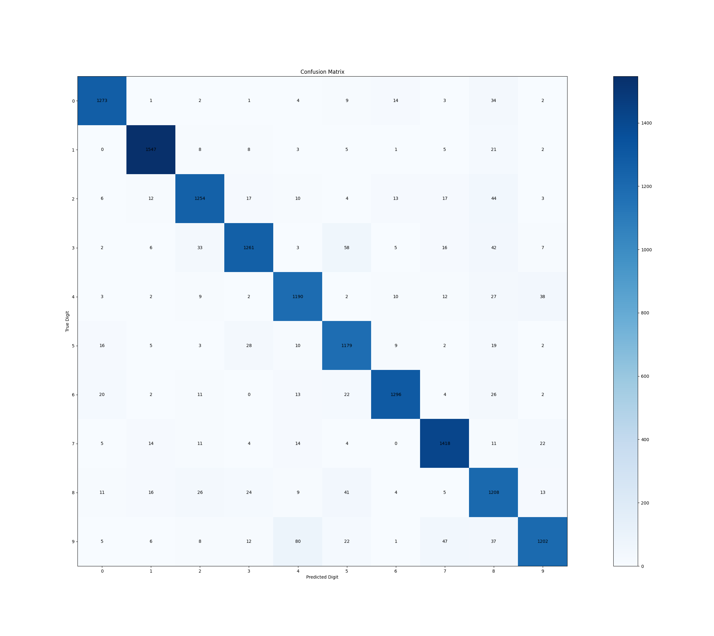
Getting to our confusion matrix, this snippet should do it:
plt.figure(figsize=(8, 6))
conf_matrix = confusion_matrix(y_test_classes, y_pred_classes)

plt.imshow(conf_matrix, cmap="Blues")
plt.colorbar()

plt.title("Confusion Matrix")
plt.xlabel("Predicted Digit")
plt.ylabel("True Digit")

for i in range(10):
    for j in range(10):
        plt.text(j, i, str(conf_matrix[i, j]), ha="center", va="center")

plt.xticks(range(10))
plt.yticks(range(10))
plt.show()
The above snippet should give us a neat confusion matrix like we see below. Again, you're free to open the image in a new tab to observe this closer.

Let's go one step further, and see the average Precision and F1 Scores of all the classes:
print("\nOverall Model Performance:")
print(
    f"Average Precision: {precision_score(y_test_classes, y_pred_classes, average='macro'):.3f}"
)
print(
    f"Average F1-score: {f1_score(y_test_classes, y_pred_classes, average='macro'):.3f}"
)
Okay, we've built a machine learning model which classifies numbers in this blog! Pretty exciting stuff. This journey took us from scratching our heads about what neural networks even are, all the way to building one that can actually recognize digits. We dove into the math (yeah, those gradients were a bit scary), but hey - now you know what's actually happening under the hood when everyone talks about "AI".
Remember how we started with just simple numbers and turned them into something our computer could understand and learn from? That's the real magic here. We're not just throwing fancy terms around - we built something that can actually learn patterns and make decisions.
Sure, this is just the beginning - there's way more to explore in machine learning. But now you've got the foundations: you understand what training really means, how models learn, and most importantly, how to tell if your model is actually doing a good job (thanks, confusion matrix!).